Microsoft Excel provides several methods for creating a header row, each designed to perform a specific task, based on the user's needs. For example, you can freeze the scrolling of a specific row so that it always remains visible on the screen, even when scrolling through the rest of the worksheet. If you want the same header to appear on multiple pages, you can configure a group of specific rows and columns to print on each page of the document. If your data is organized within a table, you can use the header row to filter the information.
Steps
Part 1 of 3: Locking a Row or Column to Always Keep It Visible
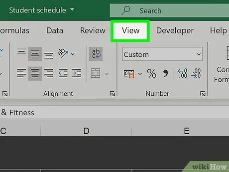
Step 1. Go to the "View" tab of the menu
If you need to keep a row of the worksheet constantly visible, even while scrolling the page, you can decide to freeze it.
Also, you can set the line to print on all pages of the document. This is a very useful trick if the worksheet is made up of several pages. For more details, see the next section of the article
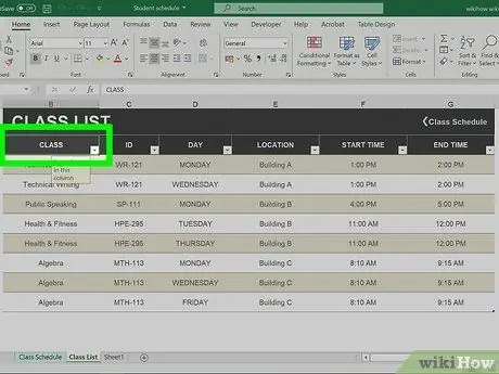
Step 2. Select the set of rows and columns you want to freeze
You can configure Excel to block the scrolling of a group of rows and columns, making them always visible to the user. To do this, you must select the cell located in the corner of the area you want to keep freely available.
For example, if you want to block the scrolling of the first row and the first column, you must select cell "B2"; this will block all the columns on the left of the selected cell and the rows above
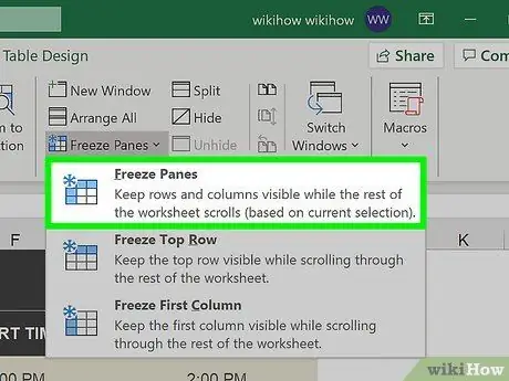
Step 3. Press the "Freeze Panes" button, then choose the "Freeze Panes" option
In this way all the rows above the selected cell and all the columns on the left will be blocked. For example, having chosen cell "B2", the first row and first column of the worksheet will always become visible on the screen.
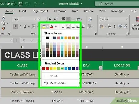
Step 4. Emphasize the header row to make it more visible (optional)
Create a visual contrast by centrally aligning the text of the cells that make up the header row. Apply a bold style to the fonts, change the background color of the cells or make them stand out by adding borders. This arrangement allows the header line of the data to always be clearly visible to the reader while consulting the spreadsheet.
Part 2 of 3: Printing the Header Row on Multiple Pages
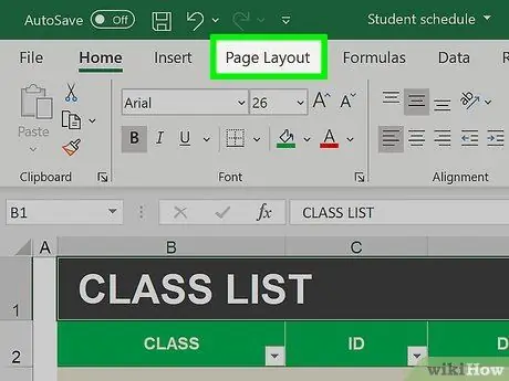
Step 1. Go to the "Page Layout" menu tab
If you need to print a spreadsheet that spans multiple pages, you can configure it so that the header row (s) are printed on all pages of the document.
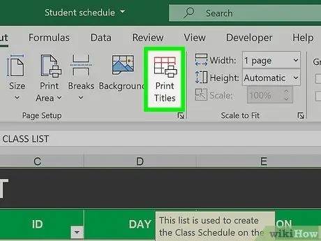
Step 2. Press the "Print Titles" button
It is available within the "Page Setup" section of the "Page Layout" tab of the menu.
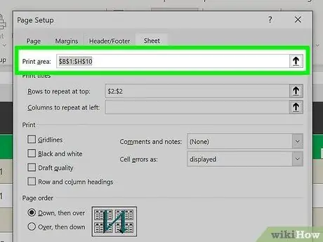
Step 3. Set the print area based on the cells containing the data
Press the button on the right of the "Print area" field, then select the cells that contain the data to be printed as a header. When selecting this piece of data, do not include cells that contain column headings or row labels.
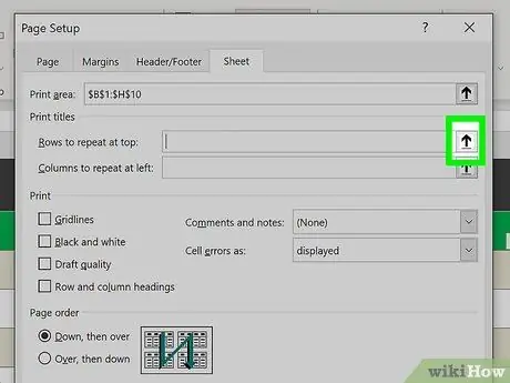
Step 4. Press the selection button for the "Rows to repeat at top" field
This step allows you to choose the row or rows to use as the header of each page.
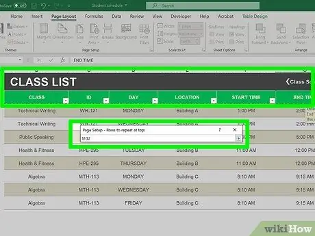
Step 5. Select the row or rows to use as the page header
The lines you choose will be printed at the top of each page that makes up the document. This is an excellent device to facilitate the reading and consultation of the data of those documents that occupy a large number of pages.
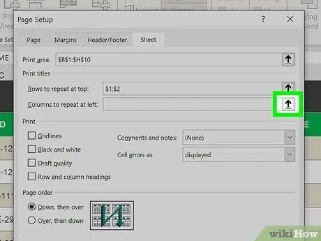
Step 6. Press the selection button for the "Columns to repeat on the left" field
This step allows you to choose the columns that will be printed on the left side of each page of the document. The chosen columns will be treated exactly like the rows selected in the previous step and will appear on all pages of the printed document.
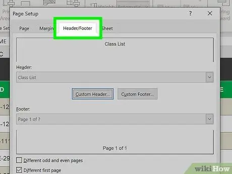
Step 7. Configure a header or footer (optional)
Go to the "Header / Footer" tab of the "Page Setup" window, then choose whether to insert a header or footer within the printed document. In the header section, you can enter your company name or document title, while, in the footer section, you can enter page numbering. This allows the user to maintain the correct order of the printed pages.
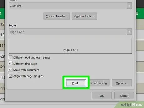
Step 8. Print the document
At this point you can send the spreadsheet to print. Excel will print the data by inserting the header rows and the columns chosen using the "Print titles" function on each of the pages of the document.
Part 3 of 3: Create a Headed Table
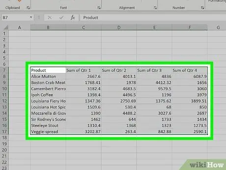
Step 1. Select the data area you want to turn into a table
By converting an area of the sheet to a table, you can use that table to manipulate and manage your data. One of the opportunities offered by tables is to be able to configure column headings. Note that the table headings are not to be confused with those of the worksheet columns or those related to printing.
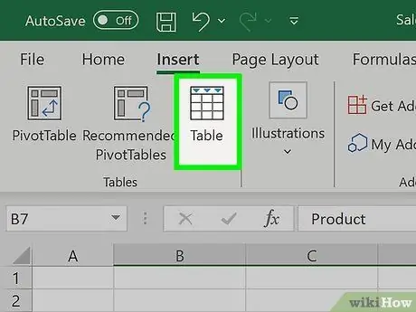
Step 2. Go to the "Insert" tab of the menu, then press the "Table" button
Confirm that the selection area relating to the data to be inserted in the table is the correct one.
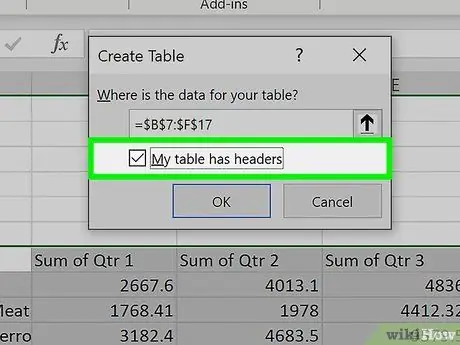
Step 3. Select the "Table with headers" checkbox, then press the "OK" button
This will create a new table using the selected data. The cells in the first row of the selection area will automatically be used as column headings.
If the "Table with headings" check button is not selected, the column headings will be created using the default Excel nomenclature. However, you can change the column headings at any time by simply selecting the relevant cell
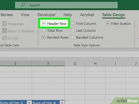
Step 4. Enable or disable the table header display
To do this, go to the "Design" tab, then select or deselect the "Header Row" checkbox. This button is located in the "Table Style Options" section of the "Design" tab.
Advice
- The "Freeze Panes" command works like a toggle. If this function is active, select it again to unlock the previously locked portion of the sheet. By selecting "Freeze Panes" again, the selected cells will be locked again.
- Most of the mistakes made using the "Freeze Panes" feature is to select the header row instead of the next one. If the result of your work is not what you want, deactivate the "Freeze Panes" function, select the line below the previous one, then reactivate the option in question.


